Interactive Visualizion with Open Altimetry & Google Earth Engine

By Philipp Arndt, Chancelor Roberts
Scripps Institution of Oceanography, University of California San Diego
Github: fliphilipp, chancelorr
Contact: ccroberts@ucsd.edu

Prerequisites¶

Concepts	Importance	Notes
pandas	Necessary	ICESat-2 data in this tutorial will appear as `geopandas` DataFrames organized within a custom class object called a `dataCollector`
numpy/matplotlib	Necessary	We will plot ICESat-2 data with `matplotlib`
rasterio	Helpful	We will plot images with `rasterio`
ICESat-2 Mission Overview	Helpful	Here is where to go to understand the ICESat-2 mission and its goals

Time to learn: 30 min.

Learning Objectives¶

Concepts	Notes
OpenAltimetry	We will learn to browse OpenAltimetry to discover ICESat-2 data, then view them as profiles or overlay them on a map
Google Earth Engine	We will learn to browse Google Earth Engine to find the closest-in-time Sentinel-2 image that is cloud-free along ICESat-2’s ground track
geemap	We will see a demonstration of the interactive mapping options available through GEEMap’s implementation of the `folium` and `ipyleaflet` python libraries
dicts	We see an example usage of Python’s dictionary data structure to organize incoming ICESat-2 data and Google Earth Engine imagery

Computing environment¶

We’ll be using the following Python libraries in this notebook:

#%matplotlib widget 
import os
import ee
import geemap
import requests
import numpy as np
import pandas as pd
import matplotlib.pylab as plt
from datetime import datetime
from datetime import timedelta
from ipywidgets import Layout
import rasterio as rio
from rasterio import plot as rioplot
from rasterio import warp

/Users/ccroberts/opt/miniforge3/envs/is2cb/lib/python3.13/site-packages/geemap/conversion.py:23: UserWarning: pkg_resources is deprecated as an API. See https://setuptools.pypa.io/en/latest/pkg_resources.html. The pkg_resources package is slated for removal as early as 2025-11-30. Refrain from using this package or pin to Setuptools<81.
  import pkg_resources

The import below is a class that I wrote myself. It helps us read and store data from the OpenAltimetry API.
If you are interested in how this works, you can find the code in utils/oa.py.

import utils.oa as oa
from utils.oa import dataCollector

Google Earth Engine Authentication and Initialization¶

GEE requires you to authenticate your access, so if ee.Initialize() does not work you first need to run ee.Authenticate(). This gives you a link at which you can use your google account that is associated with GEE to get an authorization code. Copy the authorization code into the input field and hit enter to complete authentication.

try:
    ee.Initialize()
except: 
    ee.Authenticate()
    ee.Initialize()

Downloading data from the OpenAltimetry API¶

Let’s say we have found some data that looks weird to us, and we don’t know what’s going on.

A short explanation of how I got the data:¶

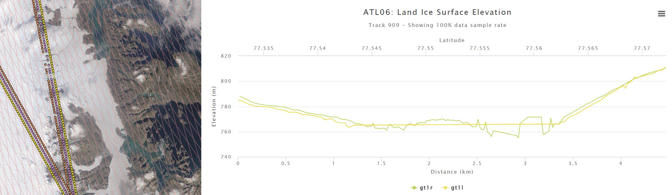
I went to openaltimetry.org and selected BROWSE ICESAT-2 DATA. Then I selected ATL 06 (Land Ice Height) on the top right, and switched the projection🌎 to Arctic. Then I selected August 22, 2021 in the calendar📅 on the bottom left, and toggled the cloud☁️ button to show MODIS imagery of that date. I then zoomed in on my region of interest.

To find out what ICESat-2 has to offer here, I clicked on SELECT A REGION on the top left, and drew a rectangle around that mysterious cloud. When right-clicking on that rectangle, I could select View Elevation profile. This opened a new tab, and showed me ATL06 and ATL08 elevations.

It looks like ATL06 can’t decide where the surface is, and ATL08 tells me that there’s a forest canopy on the Greenland Ice Sheet? To get to the bottom of this, I scrolled all the way down and selected 🛈Get API URL. The website confirms that the “API endpoint was copied to clipboard.” Now I can use this to access the data myself.

Getting the OpenAltimetry info into python¶

All we need to do is to paste the API URL that we copied from the webpage into a string. We also need to specify which beam we would like to look at. The GT1R ground track looks funky, so let’s look at that one!

# paste the API URL from OpenAltimetry below, and specify the beam you are interested in
oa_api_url = 'https://openaltimetry.earthdatacloud.nasa.gov/data/icesat2/elevation?minx=-25.4835556641541&miny=76.44321462688005&maxx=-21.976284749133928&maxy=77.33633089376721&zoom_level=5&beams=1,2,3,4,5,6&tracks=1236&date=2024-09-06&product=ATL06&mapType=arctic'
gtx = 'gt1r'

We can now initialize a dataCollector object, using the copy-pasted OpenAltimetry API URL, and the beam we would like to look at.
(Again, I defined this class in utils/oa.py to do some work for us in the background.)

is2data = dataCollector(oaurl=oa_api_url, beam=gtx, verbose=True)

Alternatively, we could use a date, track number, beam, and lat/lon bounding box as input to the dataCollector.

date = '2021-08-22'
rgt = 909
beam = 'gt1r'
latlims = [77.5326, 77.5722]
lonlims = [-23.9891, -23.9503]
is2data = dataCollector(date=date, latlims=latlims, lonlims=lonlims, track=rgt, beam=beam, verbose=True)

Note that this also constructs the API url for us.

Requesting the data from the OpenAltimetry API¶

Here we use the requestData() function of the dataCollector class, which is defined in utils/oa.py. It downloads all data products that are available on OpenAltimetry based on the inputs with which we initialized our dataCollector, and writes them to pandas dataframes.

is2data.requestData(verbose=True)

The data are now stored as data frames in our dataCollector object. To verify this, we can run the cell below.

vars(is2data)

Plotting the ICESat-2 data¶

Now let’s plot this data. Here, we are just creating an empty figure fig with axes ax.

# create the figure and axis
fig, ax = plt.subplots(figsize=[9,5])

# plot the data products
atl06, = ax.plot(is2data.atl06.lat, is2data.atl06.h, c='C0', linestyle='-', label='ATL06')
atl08, = ax.plot(is2data.atl08.lat, is2data.atl08.h, c='C2', linestyle=':', label='ATL08')
if np.sum(~np.isnan(is2data.atl08.canopy))>0:
    atl08canopy = ax.scatter(is2data.atl08.lat, is2data.atl08.h+is2data.atl08.canopy, s=2, c='C2', label='ATL08 canopy')

# add labels, title and legend
ax.set_xlabel('latitude')
ax.set_ylabel('elevation in meters')
ax.set_title('Some ICESat-2 data I found on OpenAltimetry!')
ax.legend(loc='upper left')

# add some text to provide info on what is plotted
info = 'ICESat-2 track {track:d}-{beam:s} on {date:s}\n({lon:.4f}E, {lat:.4f}N)'.format(track=is2data.track, 
                                                                                        beam=is2data.beam.upper(), 
                                                                                        date=is2data.date, 
                                                                                        lon=np.mean(is2data.lonlims), 
                                                                                        lat=np.mean(is2data.latlims))
infotext = ax.text(0.01, -0.08, info,
                   horizontalalignment='left', 
                   verticalalignment='top', 
                   transform=ax.transAxes,
                   fontsize=7,
                   bbox=dict(edgecolor=None, facecolor='white', alpha=0.9, linewidth=0))

# set the axis limits
ax.set_xlim((is2data.atl03.lat.min(), is2data.atl03.lat.max()))
ax.set_ylim((741, 818));

Let’s add the ATL03 photons to better understand what might be going on here.

atl03 = ax.scatter(is2data.atl03.lat, is2data.atl03.h, s=1, color='black', label='ATL03', zorder=-1)
ax.legend(loc='upper left')
fig.tight_layout()
display(fig)

Saving the plot to a file¶

fig.savefig('my-plot.jpg', dpi=300)

To make plots easier to produce, the dataCollector class also has a method to plot the data that we downloaded.

fig = is2data.plotData();
fig

Ground Track Stats¶

So far we have only seen the data in elevation vs. latitude space. It’s probably good to know what the scale on the x-axis is here in units that we’re familiar with.

def dist_latlon2meters(lat1, lon1, lat2, lon2):
    # returns the distance between two coordinate points - (lon1, lat1) and (lon2, lat2) along the earth's surface in meters.
    R = 6371000
    def deg2rad(deg):
        return deg * (np.pi/180)
    dlat = deg2rad(lat2-lat1)
    dlon = deg2rad(lon2-lon1)
    a = np.sin(dlat/2) * np.sin(dlat/2) + np.cos(deg2rad(lat1)) * np.cos(deg2rad(lat2)) * np.sin(dlon/2) * np.sin(dlon/2)
    c = 2 * np.arctan2(np.sqrt(a), np.sqrt(1-a))
    return R * c

lat1, lat2 = is2data.atl08.lat[0], is2data.atl08.lat.iloc[-1]
lon1, lon2 = is2data.atl08.lon[0], is2data.atl08.lon.iloc[-1]

ground_track_length = dist_latlon2meters(lat1, lon1, lat2, lon2)
print('The ground track is about %.1f kilometers long.' % (ground_track_length/1e3))

Google Earth Engine¶

Google Earth Engine (GEE) has a large catalog of geospatial raster data, which is ready for analysis in the cloud. It also comes with an online JavaScript code editor.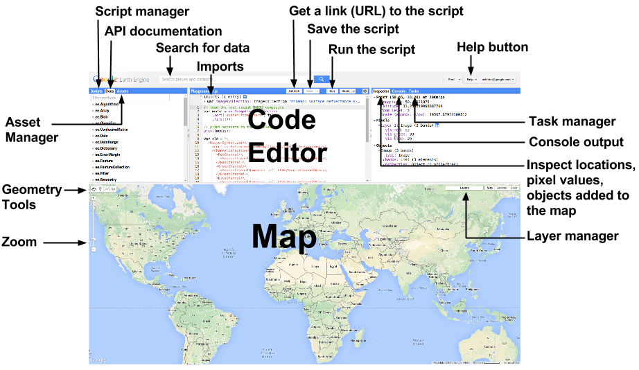
gif showing how to get to the data in OpenAltimetry

But since we all seem to be using python, it would be nice to have these capabilities available in our Jupyter comfort zone...

Thankfully, there is a python API for GEE, which we have imported using import ee earlier. It doesn’t come with an interactive map, but the python package geemap has us covered!

Show a ground track on a map¶

We can start working on our map by calling geemap.Map(). This just gives us a world map with a standard basemap.

from ipywidgets import Layout
Map = geemap.Map(layout=Layout(width='70%', max_height='450px'))
Map

Now we need to add our ICESat-2 gound track to that map. Let’s use the lon/lat coordinates of the ATL08 data product for this.
We also need to specify which Coordinate Reference System (CRS) our data is in. The longitude/latitude system that we are all quite familiar with is referenced by EPSG:4326. To add the ground track to the map we need to turn it into an Earth Engine “Feature Collection”.

ground_track_coordinates = list(zip(is2data.atl08.lon, is2data.atl08.lat))
ground_track_projection = 'EPSG:4326' # <-- this specifies that our data longitude/latitude in degrees [https://epsg.io/4326]
gtx_feature = ee.FeatureCollection(ee.Geometry.LineString(coords=ground_track_coordinates, 
                                      proj=ground_track_projection, 
                                      geodesic=True))
gtx_feature

Now that we have it in the right format, we can add it as a layer to the map.

Map.addLayer(gtx_feature, {'color': 'red'}, 'ground track')

According to the cell above this should be a red line. But we still can’t see it, because we first need to tell the map where to look for it.
Let’s calculate the center longitude and latitude, and center the map on it.

center_lon = (lon1 + lon2) / 2
center_lat = (lat1 + lat2) / 2
Map.setCenter(center_lon, center_lat, zoom=7);

So we actually couldn’t see it because it was in Greenland.
Unfortunately the basemap here doesn’t give us much more information. Let’s add a satellite imagery basemap. This is a good time to look at the layer control on the top right.

Map.add_basemap('SATELLITE') # <-- this adds a layer called 'Google Satellite'
Map.setCenter(center_lon, center_lat, zoom=7);
Map.addLayer(gtx_feature,{'color': 'red'},'ground track')

...looks like this basemap still doesn’t give us any more clues about the nature of this weird ICESat-2 data. Let’s dig deeper.

Query for Sentinel-2 images¶

Both of these Sentinel-2 satellites take images of most places on our planet at least every week or so. Maybe these images can tell us what was happening here around the same time that ICESat-2 acquired our data?

The imagery scenes live in image collections on Google Earth Engine.
You can find all collections here: https://developers.google.com/earth-engine/datasets/catalog/

The above link tells us we can find some images under 'COPERNICUS/S2_SR_HARMONIZED'.

collection_name1 = 'COPERNICUS/S2_SR_HARMONIZED'  # Landsat 8 earth engine collection 
# https://developers.google.com/earth-engine/datasets/catalog/LANDSAT_LC08_C01_T2

Access an image collection¶

To access the collection, we call ee.ImageCollection:

collection = ee.ImageCollection(collection_name1)
collection

Can we find out how many images there are in total?

number_of_scenes = collection.size()
print(number_of_scenes)

Actually, asking for the size of the collection does not do anything! 🤔

It just tells Earth Engine on the server-side that this variable refers to the size of the collection, which we may need later to do some analysis on the server. As long as this number is not needed, Earth Engine will not go through the trouble actually computing it.

To force Earth Engine to compute and get any information on the client side (our local machine / Cryocloud), we need to call .getInfo(). In this case that would be number_of_scenes = collection.size().getInfo().

# number_of_scenes = collection.size().getInfo()
number_of_scenes = 19323842
print('There are %i number of scenes in the image collection' % number_of_scenes)

Filter an image collection by location and time¶

Who wants to look at almost 20 million pictures? I don’t. So let’s try to narrow it down.
Let’s start with only images that overlap with the center of our ground track.

# the point of interest (center of the track) as an Earth Engine Geometry
point_of_interest = ee.Geometry.Point(center_lon, center_lat)

collection = collection.filterBounds(point_of_interest)

print('There are {number:d} images in the spatially filtered collection.'.format(number=collection.size().getInfo()))

Much better! Now let’s only look at images that were taken soon before or after ICESat-2 passed over this spot.

days_buffer_imagery = 6

dateformat = '%Y-%m-%d'
datetime_requested = datetime.strptime(is2data.date, dateformat)
search_start = (datetime_requested - timedelta(days=days_buffer_imagery)).strftime(dateformat)
search_end = (datetime_requested + timedelta(days=days_buffer_imagery)).strftime(dateformat)
print('Search for imagery from {start:s} to {end:s}.'.format(start=search_start, end=search_end))

collection = collection.filterDate(search_start, search_end)
print('There are {number:d} images in the spatially filtered collection.'.format(number=collection.size().getInfo()))

We can also sort the collection by date ('system:time_start'), to order the images by acquisition time.

collection = collection.sort('system:time_start')

Get image collection info¶

Again, we need to use .getInfo() to actually see any information on our end.

info = collection.getInfo()
type(info)

Let’s see what’s inside!

info.keys()

'features' sounds like it could hold information about the images we are trying to find...

len(info['features'])

A list of 34 things! Those are probably the 34 images in the collection. Let’s pick the first one and dig deeper!

feature_number = 0
info['features'][0].keys()

info['features'][feature_number]['id']

Looks like we found a reference to a Sentinel-2 image! Let’s look at the 'bands'.

for band in info['features'][feature_number]['bands']:
    print(band['id'], end=', ')

'properties' could be useful too!

info['features'][0]['properties'].keys()

That’s a lot going on right there! But 'GRANULE_ID' is probably useful. Let’s go through all our features and print the product id.

for feature in info['features']:
    print(feature['properties']['GRANULE_ID'])

Add a Sentinel-2 image to the map¶

The visible bands in Sentinel-2 are 'B2':blue, 'B3':green, 'B4':red.
So to show a “true color” RGB composite image on the map, we need to select these bands in the R-G-B order:

myImage = collection.first()
myImage_RGB = myImage.select('B4', 'B3', 'B2')
vis_params = {'min': 0.0, 'max': 10000, 'opacity': 1.0, 'gamma': 1.5}
Map.addLayer(myImage_RGB, vis_params, name='my image')
Map.addLayer(gtx_feature,{'color': 'red'},'ground track')
Map

This seems to have worked. But there’s clouds everywhere.

Calculate the along-track cloud probability¶

We need a better approach to get anywhere here. To do this, we use not only the Sentinel-2 Surface Reflectance image collection, but also merge it with the Sentinel-2 cloud probability collection, which can be accessed under COPERNICUS/S2_CLOUD_PROBABILITY.

Let’s specify a function that adds the cloud probability band to each Sentinel-2 image and calcultes the mean cloud probability in the neighborhood of the ICESat-2 ground track, then map this function over our location/date filtered collection.

def get_sentinel2_cloud_collection(is2data, days_buffer=6, gt_buffer=100):
    
    # create the area of interest for cloud likelihood assessment
    ground_track_coordinates = list(zip(is2data.atl08.lon, is2data.atl08.lat))
    ground_track_projection = 'EPSG:4326' # our data is lon/lat in degrees [https://epsg.io/4326]
    gtx_feature = ee.Geometry.LineString(coords=ground_track_coordinates,
                                     proj=ground_track_projection,
                                     geodesic=True)
    area_of_interest = gtx_feature.buffer(gt_buffer)
    
    datetime_requested = datetime.strptime(is2data.date, '%Y-%m-%d')
    start_date = (datetime_requested - timedelta(days=days_buffer)).strftime('%Y-%m-%dT%H:%M:%S')
    end_date = (datetime_requested + timedelta(days=days_buffer)).strftime('%Y-%m-%dT%H:%M:%S')
    print('Search for imagery from {start:s} to {end:s}.'.format(start=start_date, end=end_date))
    
    # Import and filter S2 SR HARMONIZED
    s2_sr_collection = (ee.ImageCollection('COPERNICUS/S2_SR_HARMONIZED')
        .filterBounds(area_of_interest)
        .filterDate(start_date, end_date))

    # Import and filter s2cloudless.
    s2_cloudless_collection = (ee.ImageCollection('COPERNICUS/S2_CLOUD_PROBABILITY')
        .filterBounds(area_of_interest)
        .filterDate(start_date, end_date))

    # Join the filtered s2cloudless collection to the SR collection by the 'system:index' property.
    cloud_collection = ee.ImageCollection(ee.Join.saveFirst('s2cloudless').apply(**{
        'primary': s2_sr_collection, 'secondary': s2_cloudless_collection,
        'condition': ee.Filter.equals(**{'leftField': 'system:index','rightField': 'system:index'})}))

    cloud_collection = cloud_collection.map(lambda img: img.addBands(ee.Image(img.get('s2cloudless')).select('probability')))
    
    def set_is2_cloudiness(img, aoi=area_of_interest):
        cloudprob = img.select(['probability']).reduceRegion(reducer=ee.Reducer.mean(), 
                                                             geometry=aoi, 
                                                             bestEffort=True, 
                                                             maxPixels=1e6)
        return img.set('ground_track_cloud_prob', cloudprob.get('probability'))
    
    return cloud_collection.map(set_is2_cloudiness)

Get this collection for our ICESat-2 data, and print all the granule IDs and associated cloudiness over the ground track.

collection = get_sentinel2_cloud_collection(is2data)
info = collection.getInfo()
for feature in info['features']:
    print('%s --> along-track cloud probability: %5.1f %%' % (feature['properties']['GRANULE_ID'],
                                                              feature['properties']['ground_track_cloud_prob']))

Filter cloudy images¶

We specify a certain cloud probability threshold, and then only keep the images that fall below it. Here we are choosing a quite aggressive value of maximum 5% cloud probability...

# filter by maximum allowable cloud probability (in percent)
MAX_CLOUD_PROB_ALONG_TRACK = 5
cloudfree_collection = collection.filter(ee.Filter.lt('ground_track_cloud_prob', MAX_CLOUD_PROB_ALONG_TRACK))
print('There are %i cloud-free scenes.' % cloudfree_collection.size().getInfo())

Sort the collection by time difference from the ICESat-2 overpass¶

Using the image property 'system:time_start' we can calculate the time difference from the ICESat-2 overpass and set it as a property. This allows us to sort the collection by it and to make sure that the first image in the collection is the closest-in-time to ICESat-2 image that is also cloud-free.

# get the time difference between ICESat-2 overpass and Sentinel-2 acquisitions, set as image property
is2time = is2data.date + 'T12:00:00'
def set_time_difference(img, is2time=is2time):
    timediff = ee.Date(is2time).difference(img.get('system:time_start'), 'second').abs()
    return img.set('timediff', timediff)
cloudfree_collection = cloudfree_collection.map(set_time_difference).sort('timediff')

Print some stats for the final collection to make sure everything looks alright.

info = cloudfree_collection.getInfo()
for feature in info['features']:
    s2datetime = datetime.fromtimestamp(feature['properties']['system:time_start']/1e3)
    is2datetime = datetime.strptime(is2time, '%Y-%m-%dT%H:%M:%S')
    timediff = s2datetime - is2datetime
    timediff -= timedelta(microseconds=timediff.microseconds)
    diffsign = 'before' if timediff < timedelta(0) else 'after'
    print('%s --> along-track cloud probability: %5.1f %%, %s %7s ICESat-2' % (feature['properties']['GRANULE_ID'],
              feature['properties']['ground_track_cloud_prob'],np.abs(timediff), diffsign))

Show the final image and ground track on the map¶

first_image_rgb = cloudfree_collection.first().select('B4', 'B3', 'B2')
Map = geemap.Map(layout=Layout(width='70%', max_height='450px'))
Map.add_basemap('SATELLITE')
Map.addLayer(first_image_rgb, vis_params, name='my image')
Map.addLayer(gtx_feature,{'color': 'red'},'ground track')
Map.centerObject(gtx_feature, zoom=12)
Map

Download images from Earth Engine¶

We can use .getDownloadUrl() on an Earth Engine image.

It asks for a scale, which is just the pixel size in meters (10 m for Sentinel-2 visible bands). It also asks for the region we would like to export; here we use a .buffer around the center.

Note - Unknown Directive

This function can only be effectively used for small download jobs because there is a request size limit. Here, we only download a small region around the ground track, and convert the image to an 8-bit RGB composite to keep file size low. For larger jobs you should use [`Export.image.toDrive`](https://developers.google.com/earth-engine/apidocs/export-image-todrive):::

# create a region around the ground track over which to download data
point_of_interest = ee.Geometry.Point(center_lon, center_lat)
buffer_around_center_meters = ground_track_length*0.52
region_of_interest = point_of_interest.buffer(buffer_around_center_meters)

# make the image 8-bit RGB
s2rgb = first_image_rgb.unitScale(ee.Number(0), ee.Number(10000)).clamp(0.0, 1.0).multiply(255.0).uint8()

# get the download URL
downloadURL = s2rgb.getDownloadUrl({'name': 'mySatelliteImage',
                                          'crs': s2rgb.projection().crs(),
                                          'scale': 10,
                                          'region': region_of_interest,
                                          'filePerBand': False,
                                          'format': 'GEO_TIFF'})
downloadURL

We can save the content of the download URL with the requests library.

response = requests.get(downloadURL)
filename = 'my-satellite-image.tif'
with open(filename, 'wb') as f:
    f.write(response.content)
print('Downloaded %s' % filename)

Open a GeoTIFF in rasterio¶

myImage = rio.open(filename)
myImage

Plot a GeoTIFF in Matplotlib¶

Now we can easily plot the image in a matplotlib figure, just using the rasterio.plot() module.

fig, ax = plt.subplots(figsize=[4,4])
rioplot.show(myImage, ax=ax);

transform the ground track into the image CRS¶

Because our plot is now in the Antarctic Polar Stereographic Coordrinate Reference System, we need to project the coordinates of the ground track from lon/lat values. The rasterio.warp.transform function has us covered. From then on, it’s just plotting in Matplotlib.

gtx_x, gtx_y = warp.transform(src_crs='epsg:4326', dst_crs=myImage.crs, xs=is2data.atl08.lon, ys=is2data.atl08.lat)
ax.plot(gtx_x, gtx_y, color='red', linestyle='-')
ax.axis('off')

display(fig)

Summary¶

🎉 Congratulations! You’ve completed this tutorial and have seen how we can put ICESat-2 photon-level data into context using Google Earth Engine and the OpenAltimetry API.

References¶

To further explore the topics of this tutorial see the following detailed documentation:

Foundations

DRAFT: Machine Learning

Example Workflows

Land Ice Applications