Author(s)
Ben Smith, Rohaiz Haris
Learning Outcomes
How different ICESat-2 land ice products (ATL14/15, ATL11, ATL06) relate to each other
Learn the basics of retrieving land ice products using icepyx
Learn how ICESat-2 land ice products can be used to study ice-surface height changes
Open, plot, and explore gridded and along-track data
Notes
Prerequisites
| Concepts | Importance | Notes |
|---|---|---|
| xarray | Necessary | ICESat-2 data in this tutorial will appear as xarray dataframes |
| numpy/matplotlib | Necessary | We will do our plotting with matplotlib |
| ICESat-2 Mission Overview | Necessary | Here is where to go to understand the ICESat-2 mission and its goals |
Time to learn: 30 min.
# import packages:
import numpy as np                   # Numeric Python
import matplotlib.pyplot as plt      # Plotting routines
import h5py                          # general HDF5 reading/writing library
import xarray as xr
from pyproj import Transformer, CRS  # libraries to allow coordinate transforms
import glob                          # Package to locate files on disk
import os                            # File-level utilities
import re                            # regular expressions for string interpretation
import icepyx as ipx                 # Package to interact with ICESat-2 online resources
import earthaccess
from matplotlib import cm
import matplotlib as mpl
#%matplotlib widgetWhat is Land Ice?
Land ice is frozen water that is grounded on land. They are formed through the accumulation of snowfall in regions where annual snowfall exceeds annual snow melt. The accumulation of snow over thousands of years leads to the compression of snow into dense ice. Over 99 percent of Earth’s land ice is present in the Antarctic and Greenland Ice Sheets, and the remaining are glaciers located in alpine regions. Land ice heights evolve with time due to ice flow and accumulation/ablation.
How ICESat-2 measures land ice height
Laser altimeters are valuable instruments for measuring land ice height across large spatial areas. ICESat-2 works by sending out photons that bounce off the ice surface; by recording how long it takes for the photons to travel to the ice and back, the satellite can calculate land ice height. ICESat-2’s 91-day repeat cycle enables the monitoring of both seasonal and annual variations in ice surface height. For more details of the ICESat-2 mission, check out the mission overview page
ATL06 provides geolocated land-ice surface heights relative to the WGS84 ellipsoid. It is derived from geolocated photons of the ATL03 product over short segments (40 m).
ATL11 provides a time-series of land-ice surface heights derived from the ATL06 product.
ATL14 is a spatially continuous gridded product of land-ice surface heights derived from the ATL11 product. ATL15 provides gridded surface height-change maps over time intervals as fine as 3 months.
The Problem
We will be looking at Svalbard in the Norwegian Arctic, focusing on the massive surge from the Austfonna ice cap. This started in 2010, and the ice cap is still adjusting to the rapid loss of ice, so we expect to see large thinning rates in the area affected by the surge. We will use the ICESat-2 ATL15 product for a look at the mass-loss pattern over the last three years.
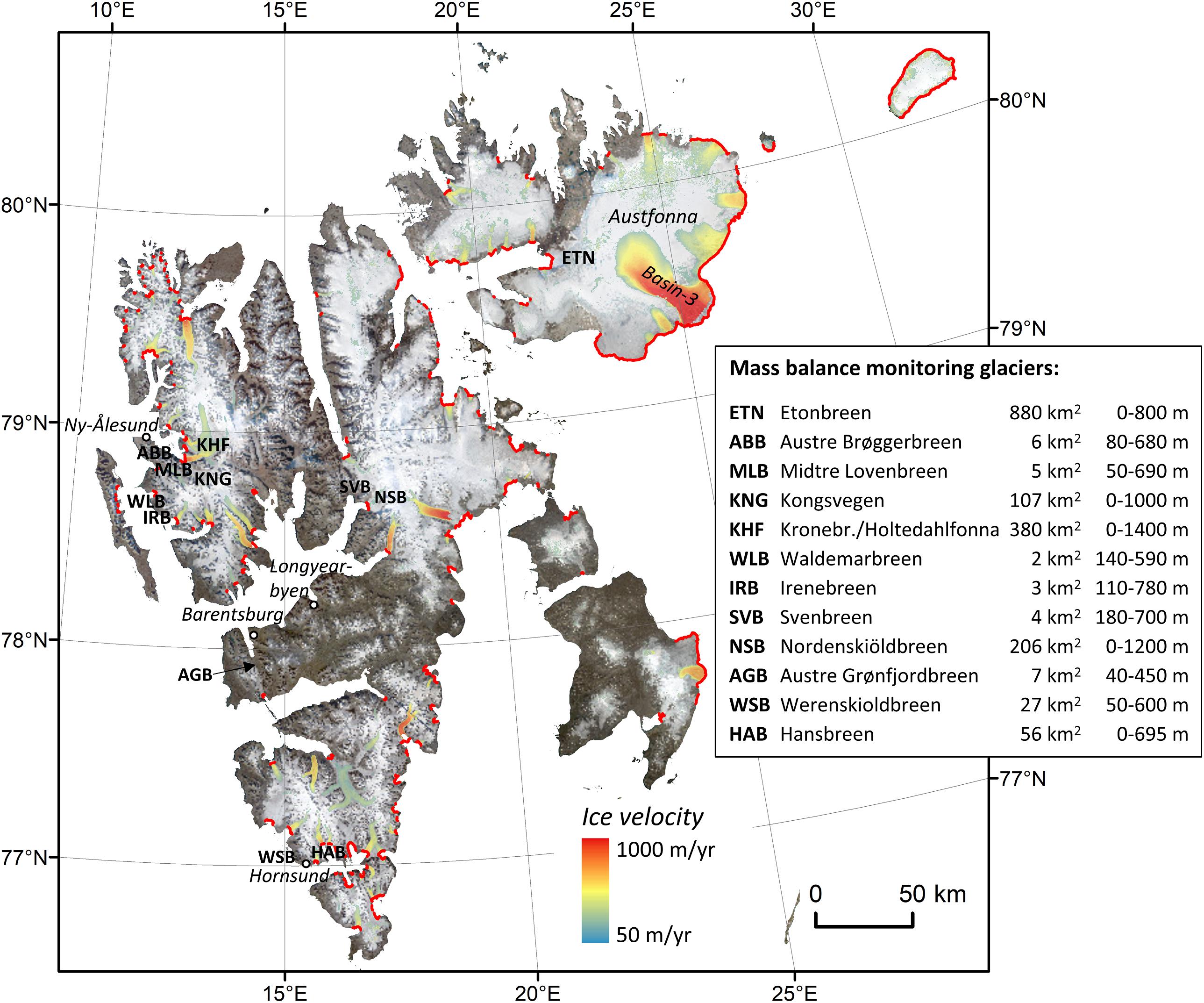
“Photo credit: Schuler et. al, Front. Earth Sci., 27 May 2020 | Schuler et al. (2020)”
ATL15
ATL15 is one of the various ICESat-2 data products. ATL15 provides various resolutions (1 km, 10 km, 20 km, and 40 km) of gridded raster data of height change at 3-month intervals, allowing for visualization of height-change patterns and calculation of integrated active subglacial lake volume change (Smith and others, 2022).
ATL14 is an accompanying high-resolution (100 m) digital elevation model (DEM) that provides spatially continuous gridded data of ice sheet surface height.
ATL14 and ATL15 are higher level products derived from lower level products (ATL11) that allow for simplified volume change calculations. However, the finest temporal resolution is 3 months which may be too coarse for certain applications. ATL14 estimates also degrade where measurements are unavailable. Potential use cases for ATL14 and ATL15 are gridded estimates of height change for ice sheet models or the creation of land ice mass balance estimates
We can use the icepyx library to access ICESat-2 data. For a deeper dive into icepyx, check out their documentation. We first query for the spatial region and the time period that we are interested in
region_a = ipx.Query('ATL15',[10, 79, 30, 81],['2019-01-01','2023-01-01'])We can visualize this spatial extent also.
region_a.visualize_spatial_extent()
Let us now place an order for the granules that are available over our spatial region and time period and download the files. This following cell will prompt you for your earthdata account username and password. Creating an account is free and can be done here.
check_fileexist = glob.glob('./data/ATL15*')
if not check_fileexist:
    order = region_a.order_granules(subset=True)
    files = order.download_granules("./data")
else:
    print("ATL15 files already exist")
Harmony job ID:  a819a598-3f0a-4dd9-8124-90888b08364e
Initial status of your harmony order request: successful
Downloading results for harmony job a819a598-3f0a-4dd9-8124-90888b08364e
data/ATL15_SV_0325_20km_004_05.nc
data/ATL15_SV_0325_40km_004_05.nc
data/ATL15_SV_0325_10km_004_05.nc
data/ATL15_SV_0325_01km_004_05.nc
ATL15 data comes in NetCDF format. Let’s take a look at the structure of these files.
f_name = glob.glob("./data/ATL15*")
f = xr.open_datatree(f_name[0])
print(f)
<xarray.DataTree>
Group: /
│ Attributes: (12/51)
│ GDAL_AREA_OR_POINT: Area
│ Conventions: CF-1.7
│ short_name: ATL15
│ level: L3B
│ title: SET_BY_META
│ description: This data set (ATL15) contains season...
│ ... ...
│ processing_level: 3B
│ references: http://nsidc.org/data/icesat2/data.html
│ project: ICESat-2 > Ice, Cloud, and land Eleva...
│ instrument: ATLAS > Advanced Topographic Laser Al...
│ platform: ICESat-2 > Ice, Cloud, and land Eleva...
│ source: Spacecraft
├── Group: /tile_stats
│ Dimensions: (y: 37, x: 10)
│ Coordinates:
│ * y (y) float64 296B -1.66e+06 -1.62e+06 ... -2.2e+05
│ * x (x) float64 80B 9.4e+05 9.8e+05 ... 1.26e+06 1.3e+06
│ Data variables:
│ N_data (y, x) float64 3kB ...
│ RMS_data (y, x) float32 1kB ...
│ RMS_bias (y, x) float32 1kB ...
│ N_bias (y, x) float64 3kB ...
│ RMS_d2z0dx2 (y, x) float32 1kB ...
│ RMS_d2zdt2 (y, x) float32 1kB ...
│ RMS_d2zdx2dt (y, x) float32 1kB ...
│ sigma_xx0 (y, x) float32 1kB ...
│ sigma_tt (y, x) float32 1kB ...
│ sigma_xxt (y, x) float32 1kB ...
│ Polar_Stereographic int8 1B ...
├── Group: /delta_h
│ Dimensions: (time: 25, y: 150, x: 42)
│ Coordinates:
│ * time (time) datetime64[ns] 200B 2019-01-01T06:00:00 ... 2...
│ * y (y) float64 1kB -1.685e+06 -1.675e+06 ... -1.95e+05
│ * x (x) float64 336B 9.15e+05 9.25e+05 ... 1.325e+06
│ Data variables:
│ Polar_Stereographic int8 1B ...
│ ice_area (time, y, x) float32 630kB ...
│ delta_h (time, y, x) float32 630kB ...
│ delta_h_sigma (time, y, x) float32 630kB ...
│ Attributes:
│ description: delta_h group includes variables describing height differen...
├── Group: /dhdt_lag1
│ Dimensions: (time: 24, y: 150, x: 42)
│ Coordinates:
│ * time (time) datetime64[ns] 192B 2019-02-15T21:45:00 ... 2...
│ * y (y) float64 1kB -1.685e+06 -1.675e+06 ... -1.95e+05
│ * x (x) float64 336B 9.15e+05 9.25e+05 ... 1.325e+06
│ Data variables:
│ Polar_Stereographic int8 1B ...
│ ice_area (time, y, x) float32 605kB ...
│ dhdt (time, y, x) float32 605kB ...
│ dhdt_sigma (time, y, x) float32 605kB ...
│ Attributes:
│ description: dhdt_lag1 group includes variables describing height differ...
...
├── Group: /METADATA
│ │ Attributes:
│ │ Description: ISO19115 Structured Metadata Represented within HDF5
│ │ iso_19139_dataset_xml: <?xml version="1.0"?>\n<gmd:DS_Series xsi:schemaL...
│ │ iso_19139_series_xml: <?xml version="1.0" encoding="UTF-8"?>\n<gmd:DS_S...
│ ├── Group: /METADATA/AcquisitionInformation
│ │ │ Attributes:
│ │ │ Description: Describe the group
│ │ ├── Group: /METADATA/AcquisitionInformation/lidar
│ │ │ Attributes:
│ │ │ Description: Describe the group
│ │ │ pulse_rate: 10000 pps
│ │ │ wavelength: 532 nm
│ │ │ identifier: ATLAS
│ │ │ type: Laser Altimeter
│ │ │ description: ATLAS on ICESat-2 determines the range between the satellit...
│ │ ├── Group: /METADATA/AcquisitionInformation/lidarDocument
│ │ │ Attributes:
│ │ │ Description: Describe the group
│ │ │ edition: Pre-Release
│ │ │ publicationDate: 12/31/17
│ │ │ title: A document describing the ATLAS instrument will be prov...
│ │ ├── Group: /METADATA/AcquisitionInformation/platform
│ │ │ Attributes:
│ │ │ Description: Describe the group
│ │ │ identifier: ICESat-2
│ │ │ description: Ice, Cloud, and land Elevation Satellite-2
│ │ │ type: Spacecraft
│ │ └── Group: /METADATA/AcquisitionInformation/platformDocument
│ │ Attributes:
│ │ Description: Describe the group
│ │ edition: 31-Dec-16
│ │ publicationDate: 31-Dec-16
│ │ title: The Ice, Cloud, and land Elevation Satellite-2 (ICESat-...
│ ├── Group: /METADATA/DataQuality
│ │ │ Attributes:
│ │ │ Description: Describe the group
│ │ │ scope: NOT_SET
│ │ ├── Group: /METADATA/DataQuality/CompletenessOmission
│ │ │ Attributes:
│ │ │ Description: Describe the group
│ │ │ evaluationMethodType: directInternal
│ │ │ measureDescription: TBD
│ │ │ nameOfMeasure: TBD
│ │ │ unitofMeasure: TBD
│ │ │ value: NOT_SET
│ │ └── Group: /METADATA/DataQuality/DomainConsistency
│ │ Attributes:
│ │ Description: Describe the group
│ │ evaluationMethodType: directInternal
│ │ measureDescription: TBD
│ │ nameOfMeasure: TBD
│ │ unitofMeasure: TBD
│ │ value: NOT_SET
│ ├── Group: /METADATA/DatasetIdentification
│ │ Attributes: (12/15)
│ │ Description: Describe the group
│ │ spatialRepresentationType: along-track
│ │ VersionID: 004
│ │ creationDate: 2025-04-08
│ │ fileName: ATL15_SV_0325_10km_004_05.nc
│ │ uuid: 20cbf825-3108-48f3-a58b-b69adbacec3a
│ │ ... ...
│ │ originatorOrganizationName: GSFC I-SIPS > ICESat-2 Science Investigator-...
│ │ abstract: The ICESat-2 ATL15 standard data product rep...
│ │ purpose: The purpose of ATL15 is to provide an IceSat...
│ │ credit: The software that generates the ATL15 produc...
│ │ status: onGoing
│ │ topicCategory: geoscientificInformation
│ ...
│ ├── Group: /METADATA/ProductSpecificationDocument
│ │ Attributes:
│ │ Description: Describe the group
│ │ ShortName: ATL15_SDP
│ │ characterSet: utf8
│ │ edition: v1.0
│ │ language: eng
│ │ publicationDate: Feb 2020
│ │ title: ICESat-2-SIPS-SPEC-4269 - ATLAS Science Algorithm Stand...
│ ├── Group: /METADATA/QADatasetIdentification
│ │ Attributes:
│ │ Description: Describe the group
│ │ abstract: An ASCII product that contains statistical information on ...
│ │ creationDate: 2025-04-09T00:30:15.000000Z
│ │ fileName: ATL15_SV_0325_10km_004_05.nc.qa
│ └── Group: /METADATA/SeriesIdentification
│ Attributes: (12/20)
│ Description: Describe the group
│ maintenanceAndUpdateFrequency: asNeeded
│ maintenanceDate: SET_BY_META
│ VersionID: 3.0
│ language: eng
│ characterSet: utf8
│ ... ...
│ credit: The software that generates the ATL15 ...
│ status: onGoing
│ format: HDF
│ formatVersion: 5
│ topicCategory: geoscientificInformation
│ mission: ICESat-2 > Ice, Cloud, and land Elevat...
├── Group: /orbit_info
│ Dimensions: (bounding_polygon_dim1: 28)
│ Coordinates:
│ * bounding_polygon_dim1 (bounding_polygon_dim1) int32 112B 1 2 3 ... 26 27 28
│ Data variables:
│ bounding_polygon_lat1 (bounding_polygon_dim1) float32 112B ...
│ bounding_polygon_lon1 (bounding_polygon_dim1) float32 112B ...
└── Group: /quality_assessment
Dimensions: (phony_dim_1: 1)
Dimensions without coordinates: phony_dim_1
Data variables:
qa_granule_fail_reason (phony_dim_1) int32 4B ...
qa_granule_pass_fail (phony_dim_1) int32 4B ...
We can see that there are many groups in this file. We’ll be plotting the delta_h data variable in this tutorial, here’s what we can learn about from these sources:
ATL14/15’s overview page: this is likely the ‘quarterly height changes’ described, but let’s dive deeper to be sure
ATL14/15’s Xarray Dataset imbedded metadata tells us a couple things: delta_h =height change at 1 km (the resolution selected earlier) and height change relative to the datum (Jan 1, 2020) surface
ATL14/15’s data dictionary: delta_h = quarterly height change at 40 km
Ok, since the data is relative to a datum, we have two options:
Difference individual time slices to subtract out the datum, like so:
(time0 - datum) - (time1 - datum) = time0 - datum - time1 + datum = time0 - time1
Subtract out the datum directly. The datum is the complementary dataset high-resolution DEM surface contained in tha accompanying dataset ATL14.
In this tutorial we’ll use the first method to look at how the ice surface height has evolved in time.
Lets look at the structure of the file
ds = xr.open_dataset("./data/ATL15_SV_0325_01km_004_05.nc",group='delta_h')
dsLets look at the difference in ice-surface height over the first quarter and plot them
fig, ax = plt.subplots(figsize=(4,5), tight_layout=True)
dhdt = ds['delta_h'][1,:,:] - ds['delta_h'][0,:,:]
extent=np.array([np.min(ds['x'])-500, np.max(ds['x'])+500, np.min(ds['y'])-500, np.max(ds['y'])+500])
cb = ax.imshow(dhdt, origin='lower', cmap='coolwarm_r', extent=extent, aspect="auto", vmin=dhdt.min(), vmax=-dhdt.min())
ax.set_xlabel('Polar Stereographic X (m)'); ax.set_ylabel('Polar Stereographic Y (m)')
plt.colorbar(cb, fraction=0.02, label='height change [m]')
plt.show()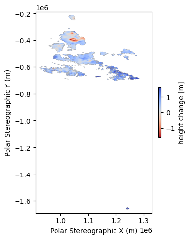
We see the difference in ice surface height for all of Svalbard. Let us zoom in to the feature of interest in Austfonna Glacier.
xlim = [1e6, 1.1e6]
ylim = [-4.5e5, -3.5e5]

fig, ax = plt.subplots(figsize=(5,4), tight_layout=True)
dhdt = ds['delta_h'][1,:,:] - ds['delta_h'][0,:,:]
extent=np.array([np.min(ds['x'])-500, np.max(ds['x'])+500, np.min(ds['y'])-500, np.max(ds['y'])+500])
cb = ax.imshow(dhdt, origin='lower', cmap='coolwarm_r', extent=extent, aspect="auto", vmin=dhdt.min(), vmax=-dhdt.min())
ax.set_xlabel('Polar Stereographic X (m)'); ax.set_ylabel('Polar Stereographic Y (m)')
ax.set_xlim(xlim)
ax.set_ylim(ylim)
plt.colorbar(cb, fraction=0.02, label='height change [m]')
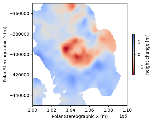
We can see a clear signal of significant decrease in height at the center of this glacier leading out into the coastline. Now what if we want to see how the ice surface height evolves over a transect? Let’s try that.
### TBC CodeTBC what we are seeing in the profiles
What if we don’t want to deal with interpolated data, and would rather see the data collected over an ICESat-2 reference ground track? Enter ATL11
ATL11
We might be interested to see where these height changes come from. ATL15 is derived from the ATL11 (slope-corrected along-track height change) product, which maps height changes for individual ICESat-2 reference tracks. It contains data for all cycles with along-track data following the Reference Ground Tracks (RGTs) and allows for the easy calculation of along-track height-change through time. However, it may not work well over complex surfaces and its 120m resolution might be too coarse for certain use cases. Potential use cases would be to make large-scale estimates of glacier and ice sheet height change.
We can use icepyx to find out what track has contributed to the height change at any given point, but for the purpose of this tutorial we shall use track 0548 which we know crosses over our region of interest. The icepyx library takes in spatial extent search parameters as latitude and longitude while our ICESat-2 data is in polar stereographic coordinates. As such, we make some coordinate transformations first in order to search for ATL11 data.
# Prepare coordinate transformations between lat/lon and the ATL15 coordinate system
crs=CRS.from_epsg(3413)
to_xy_crs=Transformer.from_crs(crs.geodetic_crs, crs)
to_geo_crs=Transformer.from_crs(crs, crs.geodetic_crs)


corners_lat, corners_lon=to_geo_crs.transform(np.array(xlim)[[0, 1, 1, 0, 0]], np.array(ylim)[[0, 0, 1, 1, 0]])
latlims=[np.min(corners_lat), np.max(corners_lat)]
lonlims=[np.min(corners_lon), np.max(corners_lon)]
Now that we’ve made the necessary coordinate transformations, let us make a query for the data we want.
region_a = ipx.Query('ATL11', [lonlims[0], latlims[0], lonlims[1], latlims[1]], ['2019-01-01','2023-01-01'], \
                          start_time='00:00:00', end_time='23:59:59', tracks = ['0548'])
We can now order and download the data.
check_fileexist = glob.glob('./data/ATL11*')
if not check_fileexist:
    region_a.avail_granules()
    order = region_a.order_granules(subset=True)
    files = order.download_granules("./data")
else:
    print("ATL11 files already exist")
Harmony job ID: 4991cafb-641d-410c-ae6f-314d466d1548
Initial status of your harmony order request: running
Downloading results for harmony job 4991cafb-641d-410c-ae6f-314d466d1548
data/ATL11_054804_0328_007_01.h5
data/ATL11_054803_0328_007_01.h5
We retrieve two files. Based on the naming convention, the ‘ATL11_054803’ file is the ascending track in the northern mid latitudes and the ‘ATL11_054804’ file is the descending track in the mid-northern-hemisphere. You can read more about the naming convention in the ATL11 user guide.
ATL11 files are in HDF5 format. We can use the glob package to find the files in the folder we’ve downloaded and the h5py package to open the ascending track file and look at its structure.
ATL11_file=glob.glob('./data/ATL11_054803*')[0]
ATL11 = h5py.File(ATL11_file)
list(ATL11.keys())
['METADATA',
'ancillary_data',
'orbit_info',
'pt1',
'pt2',
'pt3',
'quality_assessment']The ‘pt1’, ’pt2’, and ‘pt3’ groups contain data for the left, middle and right pair tracks. It’s in these tracks that we find the data. Let’s take a look at the middle beam, ‘pt2’.
list(ATL11['pt2'].keys())['cycle_number',
'cycle_stats',
'delta_time',
'h_corr',
'h_corr_sigma',
'h_corr_sigma_systematic',
'latitude',
'longitude',
'quality_summary',
'ref_pt',
'ref_surf']We are interested in ‘h_corr’, the corrected ice surface height. ‘cycle_number’ lists the cycles that are used for this file and are continually being updated as the ICESat-2 mission progresses. We only want the points over our feature of interest so let us subset the file based on our plot limits as follows.
lat = ATL11['pt2']['latitude'][:]
lon = ATL11['pt2']['longitude'][:]
h_corr = ATL11['pt2']['h_corr'][:,:]
cyc_num = ATL11['pt2']['cycle_number'][:]
h_corr[h_corr==ATL11['pt2']['h_corr'].attrs['_FillValue']]=np.nan

x_atl11,y_atl11 = to_xy_crs.transform(lat, lon)

ind = x_atl11 > xlim[0]
ind &= x_atl11 < xlim[1]
ind &= y_atl11 > ylim[0]
ind &= y_atl11 < ylim[1]
We can now go ahead and plot the 0548 track over our previous ATL15 data to understand the spatial context of our downloaded ATL11 file.
fig, ax = plt.subplots(figsize=(5,4), tight_layout=True)
ax.imshow(dhdt, origin='lower', cmap='coolwarm_r', extent=extent, aspect="auto", vmin=dhdt.min(), vmax=-dhdt.min())
#plt.gca().set_aspect(1)
plt.plot(x_atl11,y_atl11,'.')
ax.set_xlim(xlim)
ax.set_ylim(ylim)
plt.gca().set_xlabel('Polar Stereographic X (m)')
plt.gca().set_ylabel('Polar Stereographic Y (m)')

plt.tight_layout()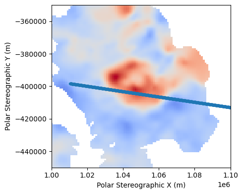
Our ATL11 file crosses over the high signal of height change. Let us see how the height profile along this track evolves with each cycle (essentially as a function of time).
fig, ax = plt.subplots(figsize=(5,4), tight_layout=True)

norm = mpl.colors.Normalize(vmin=min(cyc_num), vmax=max(cyc_num))
cmap = cm.get_cmap('viridis')


for cycle in cyc_num:
    cax = ax.plot(x_atl11[ind],h_corr[ind,cycle-3],color=cmap(norm(cycle)))
plt.colorbar(mpl.cm.ScalarMappable(cmap=cmap, norm=norm), ax=ax, label = "Cycle Number")
plt.legend()
plt.gca().set_xlabel('Polar Stereographic X (m)')
plt.gca().set_ylabel('ATL11 Height (m)')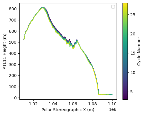
We can see that at the right and left edges of plot, the ice surface height remains mostly constant. However, in the middle (which lies over the region of strong height change signal), we can see the height decrease as the cycle number increases (and time passes).
What if we want to look at the data that went into making ATL11? Let’s take a look at ATL06.
ATL06
ATL11 data are generated by combining ALT06 data collected over the same ground track, for different cycles. We can use CMR to identify data from a specific ground track. ATL06 contains overlapping 40-meter linear segments that are fit to land and land-ice photons. It provides estimated surface heights with cm-level corrections and is a lighter and higher-level data product than the ATL03 geolocated photon product. However, its 40m resolution is too coarse for some applications and it is only designed for single surface returns. Potential use cases include making large-scale repeatable measurements of glaciers and ice sheets.
Let’s use icepyx to get the ATL06 files for the 0548 track we have been looking at. To avoid downloading too much data for this tutorial, let’s look into the ATL06 files collected over cycle 3.
region_b = ipx.Query('ATL06', spatial_extent=[lonlims[0], latlims[0], lonlims[1], latlims[1]], date_range=['2019-01-01','2023-01-01'], \
    cycles = ["03"], tracks=['0548'])
check_fileexist = glob.glob('./data/*ATL06*')
if not check_fileexist:
region_b.avail_granules()
order = region_b.order_granules(subset=True)
files = order.download_granules("./data")
else:
print("ATL06 files already exist")
Harmony job ID: 28dab34d-2d94-4459-acba-cd4c1f13bd43
Initial status of your harmony order request: running
Downloading results for harmony job 28dab34d-2d94-4459-acba-cd4c1f13bd43
data/127892349_ATL06_20190504033140_05480303_007_01_subsetted.h5
data/127892350_ATL06_20190504033705_05480304_007_01_subsetted.h5
Now that we have our ATL06 files, let’s take a look at the structure of one of our files.
ATL06_file=glob.glob('./data/*ATL06*0303*')[0]
ATL06 = h5py.File(ATL06_file)
list(ATL06.keys())
['METADATA',
'ancillary_data',
'gt1l',
'gt1r',
'gt2l',
'gt2r',
'gt3l',
'gt3r',
'orbit_info',
'quality_assessment']The ‘gtxx’ tracks refer to the ground tracks for the six beams on ICESat-2. Each ground track is numbered according to the pattern of tracks on the ground from left to right (GT1L, GT1R, GT2L, GT2R, GT3L, GT3R). The labeling was chosen such that the beam names do not change when the observatory orientation changes. Let us take a look at the beam data for GT2R, which resides in the ‘land_ice_segments’ group.
list(ATL06['gt2r']['land_ice_segments'].keys())['atl06_quality_summary',
'bias_correction',
'delta_time',
'dem',
'fit_statistics',
'fpb_warning_flag',
'geophysical',
'ground_track',
'h_li',
'h_li_sigma',
'latitude',
'longitude',
'segment_id',
'sigma_geo_h']We are interested in ‘h_li’, the land ice height. Let’s plot the ground tracks over our ATL15 data.
lat = ATL06['gt2r']['land_ice_segments']['latitude'][:]
lon = ATL06['gt2r']['land_ice_segments']['longitude'][:]
h_li = ATL06['gt2r']['land_ice_segments']['h_li'][:]
h_li[h_li==ATL06['gt2r']['land_ice_segments']['h_li'].attrs['_FillValue']]=np.nan

x_atl06,y_atl06 = to_xy_crs.transform(lat, lon)
fig, ax = plt.subplots(figsize=(5,4), tight_layout=True)
ax.imshow(dhdt, origin='lower', cmap='coolwarm_r', extent=extent, aspect="auto", vmin=dhdt.min(), vmax=-dhdt.min())
#plt.gca().set_aspect(1)
plt.plot(x_atl06,y_atl06,'.')
ax.set_xlim(xlim)
ax.set_ylim(ylim)
plt.gca().set_xlabel('Polar Stereographic X (m)')
plt.gca().set_ylabel('Polar Stereographic Y (m)')
plt.tight_layout()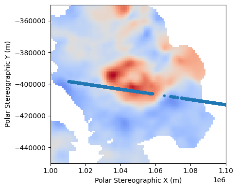
We can now plot the ATL06 data over our ATL11 data for the third cycle and see how they compare.
fig, ax = plt.subplots(figsize=(5,4), tight_layout=True)

ax.plot(x_atl11[ind],h_corr[ind,0], label="ATL11")
ax.plot(x_atl06,h_li, label = "ATL06")
plt.legend()
plt.gca().set_xlabel('Polar Stereographic X (m)')
plt.gca().set_ylabel('Ice Surface height (m)')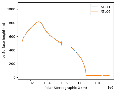
What gives? It’s likely that some of the ATL06 data is bad. Fortunately, ATL06 comes with a quality flag (atl06_quality_summary) that identifies segments that are likely good (zero means no problems). Let’s filter out the bad data and try this again with the good data.
fig, ax = plt.subplots(figsize=(5,4), tight_layout=True)

good=(ATL06['gt2r']['land_ice_segments']['atl06_quality_summary'][:]==0)
if np.any(good):
        plt.plot(x_atl06[good],h_li[good],'.', label = "ATL06")
plt.plot(x_atl11[ind],h_corr[ind,0], label = "ATL11")
plt.legend()
plt.gca().set_xlabel('Polar Stereographic X (m)')
plt.gca().set_ylabel('Ice Surface Height (m)')
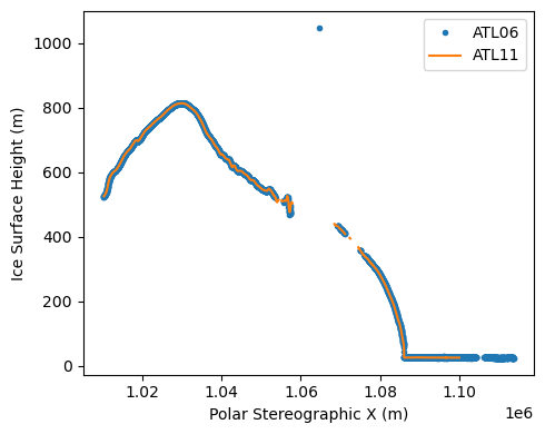
Great success! We see that our ATL06 data is colocated with the ATL11 data now.
TBC Conclusion
We have briefly explored how to use different ICESat-2 land ice products to study ice mass loss in Svalbard and how to interact with these datasets. It is worth noting that ICESat-2 land ice products have been used in many other ways, here is a list of some publications that have used these products.
TBC papers that have used these datasets and are good references
References
Smith, B., Fricker, H. A., Holschuh, N., Gardner, A. S., Adusumilli, S., Brunt, K. M., et al. (2019). Land ice height-retrieval algorithm for NASA’s ICESat-2 photon-counting laser altimeter. Remote Sensing of Environment, 233, 111352. doi:Smith et al. (2019)
Smith, B., T. Sutterley, S. Dickinson, B. P. Jelley, D. Felikson, T. A. Neumann, H. A. Fricker, A. Gardner, L. Padman, T. Markus, N. Kurtz, S. Bhardwaj, D. Hancock, and J. Lee. (2022). ATLAS/ICESat-2 L3B Gridded Antarctic and Arctic Land Ice Height Change, Version 2 [Data Set]. Boulder, Colorado USA. NASA National Snow and Ice Data Center Distributed Active Archive Center. Smith et al. (2022).
Smith, B., T. Sutterley, S. Dickinson, B. P. Jelley, D. Felikson, T. A. Neumann, H. A. Fricker, A. Gardner, L. Padman, T. Markus, N. Kurtz, S. Bhardwaj, D. Hancock, and J. Lee. “ATL15 Data Dictionary (V01).” National Snow and Ice Data Center (NSIDC), 2021-11-29. https://
Sauthoff, W., L. Lopez, J. Scheick, T. Snow. IS2-ATL15 Surface-Height Anomalies. CryoCloud: Accelerating discovery for NASA Cryosphere communities. Retrieved August 20, 2025, from https://
- Schuler, T. V., Kohler, J., Elagina, N., Hagen, J. O. M., Hodson, A. J., Jania, J. A., Kääb, A. M., Luks, B., Małecki, J., Moholdt, G., Pohjola, V. A., Sobota, I., & Van Pelt, W. J. J. (2020). Reconciling Svalbard Glacier Mass Balance. Frontiers in Earth Science, 8. 10.3389/feart.2020.00156