Author(s)
Karina Zikan, Zach Fair
Learning Outcomes
Gain experience in working with SlideRule to access and pre-process ICESat-2 data
Learn how to use projections and interpolation to compare ICESat-2 track data with gridded raster products
Develop a general understanding of how to measure snow depths with LiDAR, and learn about opportunities and challenges when using ICEsat-2 along-track products
Background
How do we measure snow depth with LiDAR?
LiDAR is a useful tool for collecting high resolution snow depth maps over large spatial areas.
Snow depth is measured from LiDAR by differencing a snow-free LiDAR map from a snow-covered LiDAR map of the same area of interest.
TODO: Insert Figure 6 from Deems et al. here
TODO: Insert Figure 7b from Deems et al
Can we do this with ICESat-2?
Yes! By differencing snow-covered ICESat-2 transects from snow-free maps, we can calculate snow depth!
Performing the calculation with ICESat-2 is a little different from other LiDAR snow depth methods, given that ICESat-2 is a transect of points rather than gridded raster data. ICESat-2 also has sparse coverage in the mid-latitudes, so generating an effective snow-covered or snow-free map will be difficult.
Because of these limitations, we need an independently-collected snow-free map of a region of interest for comparison. We also need to process the snow-free data into a form that can be differenced from snow-on ICESat-2 data.
In this tutorial, we will show an example of how to compare ICESat-2 data to raster data.
TODO: Add Karina’s image over Dry Creek
What do we need to calculate snow depth from ICESat-2?
A region of interest, where snow-free (and snow-covered, for validation) digital elevation models (DEMs) are available.
ICESat-2 data, ideally from one of the lower-level products (ATL03, ATL06, ATL08, Sliderule Earth).
A snow-free reference DEM for the snow depth calculation.
What do we need to consider when comparing ICESat-2 and raster data?
Geolocation: To obtain usable results, it is important that we properly align the snow-free raster data with ICESat-2. Even small offsets can create large errors that worsen in rugged terrain.
TODO: Add Figure 9 from Nuth and Kabb
Vegetation: Incorrectly categorized vegetation returns can positively bias ground or snow surface height estimation. Additionally, dense vegetation can reduce the number of photon returns, thereby increasing uncertainty in our height estimates.
Slope Effects: Rugged terrain increases uncertainty in ICESat-2 returns and increases the impact of geolocation offsets between ICESat-2 and raster data. Additionally, steep slopes can negatively bias ground or snow surface height estimates.
Computing Environment
We’ll be using the following open source Python libraries in this notebook:
import numpy as np
import pandas as pd
import geopandas as gpd
import rioxarray as rxr
import matplotlib.pyplot as plt
from sliderule import icesat2, sliderule
from scipy.interpolate import RectBivariateSpline
Data
We will use SlideRule to acquire customized ATL06 data. Specific customizations that we will implement include footprint averaging (i.e., along-track sampling rate) and photon identification (signal/noise and ground/vegetation).
We will look at snow depth data over Upper Kuparuk/Toolik (UKT) on the Arctic North Slope of Alaska. Because UKT is a relatively flat region with little vegetation, we should expect good agreement between ICESat-2 and our rasters of interest.
Initialize SlideRule
icesat2.init("slideruleearth.io")Warning, this environment is using an outdated client (v4.19.1). The code will run but some functionality supported by the server (v4.20.0) may not be available.
TrueDefine Region of Interest
After we initialize SlideRule, we define our region of interest. Notice that there are two options given below. This is because SlideRule accepts either the coordinates of a box/polygon or a geoJSON for its region input.
We are going to use the bounding box method in this tutorial, but the syntax for the geoJSON method is included for the user’s reference.
# Define region of interest over Toolik, Alaska
region = [{"lon":-149.5992624418217, "lat":68.63358948385529},
          {"lon":-149.5954459662985, "lat":68.60200878043223},
          {"lon":-149.2821268688734, "lat":68.60675802967609},
          {"lon":-149.2855031235162, "lat":68.63834638180673},
          {"lon":-149.5992624418217, "lat":68.63358948385529}]

print(region)
[{'lon': -149.5992624418217, 'lat': 68.63358948385529}, {'lon': -149.5954459662985, 'lat': 68.60200878043223}, {'lon': -149.2821268688734, 'lat': 68.60675802967609}, {'lon': -149.2855031235162, 'lat': 68.63834638180673}, {'lon': -149.5992624418217, 'lat': 68.63358948385529}]
Build SlideRule Request
Now we are going to build our SlideRule request by defining ICESat-2 parameters.
Since we want something close to the ATL06 product, we will use the icesat2.atl06p() function in this tutorial. You can find other SlideRule functions and more detail on the icesat2.atl06p() function on the SlideRule API reference. (TODO: Add link to API reference)
We won’t use every parameter in this tutorial, but here is a reference list for some of them. More information can be found in the SlideRule users guide (TODO: Add link to users guide)
## Build SlideRule request
# Define parameters (described below)
parms = {
    "poly": region,
    "srt": icesat2.SRT_LAND,
    "cnf": icesat2.CNF_SURFACE_HIGH,
    "atl08_class": ["atl08_ground"],
    "ats": 5.0,
    "len": 20.0,
    "res": 10.0,
    "maxi": 5
}

# Calculated ATL06 dataframe
is2_df = icesat2.atl06p(parms)

# Print SlideRule output
print(is2_df.head())
gt cycle pflags h_sigma spot \
time
2018-10-20 00:56:22.190402560 50 1 0 0.058245 2
2018-10-20 00:56:22.191812864 50 1 0 0.043303 2
2018-10-20 00:56:22.193223680 50 1 0 0.035662 2
2018-10-20 00:56:22.194635776 50 1 0 0.037516 2
2018-10-20 00:56:22.196046080 50 1 0 0.039337 2
w_surface_window_final region h_mean \
time
2018-10-20 00:56:22.190402560 3.0 3 954.390111
2018-10-20 00:56:22.191812864 3.0 3 954.540931
2018-10-20 00:56:22.193223680 3.0 3 954.353795
2018-10-20 00:56:22.194635776 3.0 3 954.267078
2018-10-20 00:56:22.196046080 3.0 3 954.076347
n_fit_photons dh_fit_dx rms_misfit \
time
2018-10-20 00:56:22.190402560 27 0.051936 0.300781
2018-10-20 00:56:22.191812864 25 -0.026959 0.216516
2018-10-20 00:56:22.193223680 27 -0.011005 0.185165
2018-10-20 00:56:22.194635776 29 -0.010565 0.201655
2018-10-20 00:56:22.196046080 31 -0.019765 0.218579
segment_id y_atc rgt x_atc \
time
2018-10-20 00:56:22.190402560 381674 -4502.958984 327 7650522.0
2018-10-20 00:56:22.191812864 381675 -4502.944824 327 7650532.0
2018-10-20 00:56:22.193223680 381675 -4502.937012 327 7650542.0
2018-10-20 00:56:22.194635776 381676 -4502.930664 327 7650552.0
2018-10-20 00:56:22.196046080 381676 -4502.927734 327 7650562.0
geometry
time
2018-10-20 00:56:22.190402560 POINT (-149.49734 68.60363)
2018-10-20 00:56:22.191812864 POINT (-149.49737 68.60372)
2018-10-20 00:56:22.193223680 POINT (-149.4974 68.60381)
2018-10-20 00:56:22.194635776 POINT (-149.49743 68.6039)
2018-10-20 00:56:22.196046080 POINT (-149.49745 68.60399)
Subsetting the Data
One may notice that the algorithm took a long time to generate the GeoDataFrame. That is because (i) our region of interest was rather large and (ii) we obtained all ICESat-2 tracks in the ROI since its launch (2018).
For the sake of interest, let’s take a look at all of the ICESat-2 tracks over Upper Kuparuk/Toolik.
import contextily as ctx
from shapely.geometry import Polygon

# Convert region to a Polygon
coords = [(point["lon"], point["lat"]) for point in region]
polygon = Polygon(coords)
region_gdf = gpd.GeoDataFrame([1], geometry=[polygon], crs="EPSG:4326")

# Reproject to Web Mercator for contextily
is2_df_mercator = is2_df.to_crs(epsg=3857)
region_mercator = region_gdf.to_crs(epsg=3857)


fig, ax = plt.subplots(figsize=(12, 8))
# Plot surface height
is2_df_mercator.plot(column='h_mean',
                  ax=ax,
                  cmap='viridis',
                  legend=True,
                  markersize=10,
                  alpha=0.8)

# Plot the region bounding box
region_mercator.plot(ax=ax,
                     facecolor='none',
                     edgecolor='red',
                     linewidth=2)

# Add ESRI World Imagery basemap
ctx.add_basemap(ax,
                crs=is2_df_mercator.crs,
                source=ctx.providers.Esri.WorldImagery)
plt.tight_layout()
plt.show()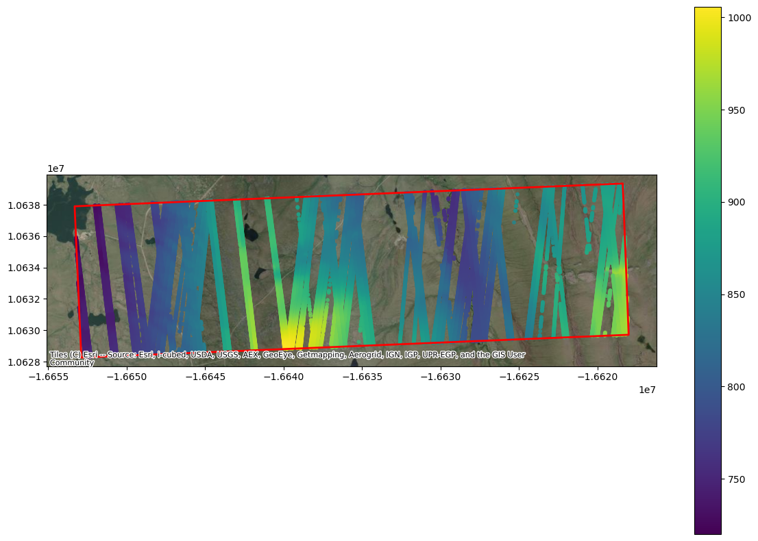
It is cool to see all of the available data, but we only have snow-free lidar DEMs available from March 2022. So, we are going to subset the data to include one ICESat-2 track (RGT 152) in March 2023.
# Subset ICESat-2 data to single RGT, time of year
is2_df_subset = is2_df[is2_df['rgt']==152]
is2_df_subset = is2_df_subset.loc['2023-03-31']

# Display top of dataframe
print(is2_df_subset.head())
gt cycle pflags h_sigma spot \
time
2023-03-31 08:03:54.300458240 10 19 0 0.036000 1
2023-03-31 08:03:54.301870848 10 19 0 0.038032 1
2023-03-31 08:03:54.303283200 10 19 0 0.041716 1
2023-03-31 08:03:54.304697600 10 19 0 0.050364 1
2023-03-31 08:03:54.306111744 10 19 0 0.048279 1
w_surface_window_final region h_mean \
time
2023-03-31 08:03:54.300458240 3.0 5 837.299826
2023-03-31 08:03:54.301870848 3.0 5 836.776278
2023-03-31 08:03:54.303283200 3.0 5 836.143292
2023-03-31 08:03:54.304697600 3.0 5 835.636543
2023-03-31 08:03:54.306111744 3.0 5 835.219543
n_fit_photons dh_fit_dx rms_misfit \
time
2023-03-31 08:03:54.300458240 51 -0.047823 0.252085
2023-03-31 08:03:54.301870848 52 -0.053057 0.273711
2023-03-31 08:03:54.303283200 41 -0.073967 0.265001
2023-03-31 08:03:54.304697600 34 -0.032487 0.293191
2023-03-31 08:03:54.306111744 40 -0.048137 0.301158
segment_id y_atc rgt x_atc \
time
2023-03-31 08:03:54.300458240 620001 -20939.156250 152 12418799.0
2023-03-31 08:03:54.301870848 620002 -20939.173828 152 12418809.0
2023-03-31 08:03:54.303283200 620002 -20939.193359 152 12418819.0
2023-03-31 08:03:54.304697600 620003 -20939.203125 152 12418829.0
2023-03-31 08:03:54.306111744 620003 -20939.205078 152 12418839.0
geometry
time
2023-03-31 08:03:54.300458240 POINT (-149.35922 68.63719)
2023-03-31 08:03:54.301870848 POINT (-149.35924 68.6371)
2023-03-31 08:03:54.303283200 POINT (-149.35927 68.63701)
2023-03-31 08:03:54.304697600 POINT (-149.3593 68.63693)
2023-03-31 08:03:54.306111744 POINT (-149.35933 68.63684)
Sample the Lidar DTM to ICESat-2 ground track
The ICESat-2 data is ready to go! Now it’s time to load the airborne lidar data, and co-register it with ICESat-2.
The lidar data used here is from the University of Alaska, Fairbanks (UAF). The UAF lidar obtains snow-on and snow-off DEMs/digital terrain models (DTMs) with a 1064 nm (near-infrared) laser, from which it can also derive snow depth.
UAF lidar rasters normally have a spatial resolution of 0.5 m, which can take a long time to process. As a compromise between computation speed and resolution, we will coarsen the rasters to 3 m resolution.
The best way to handle lidar DEMs/DTMs is through rioxarray:
TODO: Access UAF lidar data without needing it locally.
import earthaccess
earthaccess.login(strategy='interactive', persist=True)
auth = earthaccess.login()
# Coordinates for SW/NE corners
lon_min = min([coord[0] for coord in coords])
lat_min = min([coord[1] for coord in coords])
lon_max = max([coord[0] for coord in coords])
lat_max = max([coord[1] for coord in coords])
# Data query for lidar point clouds over Fairbanks, AK
results = earthaccess.search_data(
short_name='SNEX23_Lidar',
bounding_box = (lon_min, lat_min, lon_max, lat_max),
temporal = ('2023-03-13', '2023-03-14')
)# File paths for UAF rasters (TODO: Add lidar files, and update names)
tifpath = "/your/path/here"
f_snow_off = f"{tifpath}/uaf_lidar_snowoff.tif"
f_snow_on = f"{tifpath}/uaf_lidar_snowon.tif"
# Load files as rioxarray datasets
lidar_snow_off = rxr.open_rasterio(f_snow_off)
lidar_snow_on = rxr.open_rasterio(f_snow_on)---------------------------------------------------------------------------
KeyError Traceback (most recent call last)
File ~/micromamba/envs/icesat2-cookbook-dev/lib/python3.13/site-packages/xarray/backends/file_manager.py:219, in CachingFileManager._acquire_with_cache_info(self, needs_lock)
218 try:
--> 219 file = self._cache[self._key]
220 except KeyError:
File ~/micromamba/envs/icesat2-cookbook-dev/lib/python3.13/site-packages/xarray/backends/lru_cache.py:56, in LRUCache.__getitem__(self, key)
55 with self._lock:
---> 56 value = self._cache[key]
57 self._cache.move_to_end(key)
KeyError: [<function open at 0x7f993c1e6fc0>, ('/your/path/here/uaf_lidar_snowoff.tif',), 'r', (('sharing', False),), 'f8627a90-c090-4e6f-a867-7a2d2892a6ed']
During handling of the above exception, another exception occurred:
CPLE_OpenFailedError Traceback (most recent call last)
File rasterio/_base.pyx:310, in rasterio._base.DatasetBase.__init__()
File rasterio/_base.pyx:221, in rasterio._base.open_dataset()
File rasterio/_err.pyx:359, in rasterio._err.exc_wrap_pointer()
CPLE_OpenFailedError: /your/path/here/uaf_lidar_snowoff.tif: No such file or directory
During handling of the above exception, another exception occurred:
RasterioIOError Traceback (most recent call last)
Cell In[9], line 7
4 f_snow_on = f"{tifpath}/uaf_lidar_snowon.tif"
6 # Load files as rioxarray datasets
----> 7 lidar_snow_off = rxr.open_rasterio(f_snow_off)
8 lidar_snow_on = rxr.open_rasterio(f_snow_on)
File ~/micromamba/envs/icesat2-cookbook-dev/lib/python3.13/site-packages/rioxarray/_io.py:1135, in open_rasterio(filename, parse_coordinates, chunks, cache, lock, masked, mask_and_scale, variable, group, default_name, decode_times, decode_timedelta, band_as_variable, **open_kwargs)
1133 else:
1134 manager = URIManager(file_opener, filename, mode="r", kwargs=open_kwargs)
-> 1135 riods = manager.acquire()
1136 captured_warnings = rio_warnings.copy()
1138 # raise the NotGeoreferencedWarning if applicable
File ~/micromamba/envs/icesat2-cookbook-dev/lib/python3.13/site-packages/xarray/backends/file_manager.py:201, in CachingFileManager.acquire(self, needs_lock)
186 def acquire(self, needs_lock: bool = True) -> T_File:
187 """Acquire a file object from the manager.
188
189 A new file is only opened if it has expired from the
(...) 199 An open file object, as returned by ``opener(*args, **kwargs)``.
200 """
--> 201 file, _ = self._acquire_with_cache_info(needs_lock)
202 return file
File ~/micromamba/envs/icesat2-cookbook-dev/lib/python3.13/site-packages/xarray/backends/file_manager.py:225, in CachingFileManager._acquire_with_cache_info(self, needs_lock)
223 kwargs = kwargs.copy()
224 kwargs["mode"] = self._mode
--> 225 file = self._opener(*self._args, **kwargs)
226 if self._mode == "w":
227 # ensure file doesn't get overridden when opened again
228 self._mode = "a"
File ~/micromamba/envs/icesat2-cookbook-dev/lib/python3.13/site-packages/rasterio/env.py:463, in ensure_env_with_credentials.<locals>.wrapper(*args, **kwds)
460 session = DummySession()
462 with env_ctor(session=session):
--> 463 return f(*args, **kwds)
File ~/micromamba/envs/icesat2-cookbook-dev/lib/python3.13/site-packages/rasterio/__init__.py:356, in open(fp, mode, driver, width, height, count, crs, transform, dtype, nodata, sharing, opener, **kwargs)
353 path = _parse_path(raw_dataset_path)
355 if mode == "r":
--> 356 dataset = DatasetReader(path, driver=driver, sharing=sharing, **kwargs)
357 elif mode == "r+":
358 dataset = get_writer_for_path(path, driver=driver)(
359 path, mode, driver=driver, sharing=sharing, **kwargs
360 )
File rasterio/_base.pyx:312, in rasterio._base.DatasetBase.__init__()
RasterioIOError: /your/path/here/uaf_lidar_snowoff.tif: No such file or directoryIt is not immediately obvious, but the uAF rasters are in a different spatial projection than ICESat-2. UAF is in EPSG:32606, and ICESat-2 is in WGS84/EPSG:4326.
In order to directly compare these two datasets, we are going to add reprojected coordinates to the ICESat-2 GeoDataFrame. In essence, we will go from latitude/longitude to northing/easting. Luckily, there is an easy way to do this with GeoPandas, specifically with the geopandas.to_crs() function.
# Initialize ICESat-2 coordinate projection
is2_df_subset = is2_df_subset.set_crs("EPSG:4326")

# Change to EPSG:32606
is2_df_subset = is2_df_subset.to_crs("EPSG:32606")

# Display top of dataframe
print(is2_df_subset.head())
Co-register rasters and ICESat-2
Now, we are going to co-register both rasters to the queried ICESat-2 data. The function below is fairly long, but the gist is that we a re using a spline interpolant to match both the snow-off UAF data (surface height) and UAF snow depths with ICESat-2 surface heights. The resulting GeoDataFrame will have both ICESat-2 and UAF data in it.
# Make coregistration function
def coregister_is2(lidar_snow_off, lidar_snow_on, is2_df):
    """
    Co-registers UAF data with ICESat-2 data with a rectangular
    bivariate spline.

    Parameters
    ------------
    lidar_snow_off: rioxarray dataset
        Lidar DEM/DTM in rioxarray format.
    lidar_snow_on: rioxarray dataset
        Lidar-derived snow depth in rioxarray format.
    is2_df: GeodataFrame
        GeoDataFrame for the ICESat-2 data generated with SlideRule.

    Returns
    ------------
    is2_uaf_df: GeoDataFrame
        Contains the coordinate and elevation data that matches best
        between ICESat-2 and UAF.
    """

    # Helper function to prepare lidar data
    def prepare_lidar_data(raster):
        coords_x = np.array(raster.x)
        coords_y = np.array(raster.y)
        values = np.array(raster.sel(band=1))[::-1, :]
        values[np.isnan(values)] = -9999
        return coords_x, coords_y, values

    # Get coordinates and height/depth values from lidar data
    x0, y0, dem_heights = prepare_lidar_data(lidar_snow_off)
    xs, ys, dem_depths = prepare_lidar_data(lidar_snow_on)

    # Generate interpolators
    interp_height = RectBivariateSpline(y0[::-1], x0, dem_heights)
    interp_height = RectBivariateSpline(ys[::-1], xs, dem_depths)

    # Pre-filter IS2 data to bounds (apply once instead of per beam)
    x_bounds = (is2_df.geometry.x > np.min(x0)) & (is2_df.geometry.x < np.max(x0))
    y_bounds = (is2_df.geometry.y > np.min(y0)) & (is2_df.geometry.y < np.max(y0))
    is2_filtered = is2_df[x_bounds & y_bounds].copy()

    if is2_filtered.empty:
        print('Error with GeoDataFrame or raster bounds.')
        return gpd.GeoDataFrame()

    # Extract coordinates once
    xn = is2_filtered.geometry.x.values
    yn = is2_filtered.geometry.y.values

    # Estimate lidar height and snow depth at the ICESat-2 coordinates
    lidar_heights = interp_height(yn, xn, grid=False)
    lidar_snow_depths = interp_depth(yn, xn, grid=False)

    # Create result DataFrame in one operation
    is2_uaf_df = gpd.GeoDataFrame({
        'x': xn,
        'y': yn,
        'time': is2_filtered.index.values,
        'beam': is2_filtered['gt'].values,
        'lidar_height': lidar_heights,
        'lidar_snow_depth': lidar_snow_depths,
        'is2_height': is2_filtered['h_mean'].values,
        'h_sigma': is2_filtered['h_sigma'].values,
        'dh_fit_dx': is2_filtered['dh_fit_dx'].values
    })

    # Add coordinate transformation
    transformer = Transformer.from_crs("EPSG:32606", "EPSG:4326", always_xy=True)
    is2_uaf_df['lon'], is2_uaf_df['lat'] = transformer.transform(
        is2_uaf_df['x'], is2_uaf_df['y']
    )

    return is2_uaf_df
# Co-locate ICESat-2 and UAF using the above function
is2_uaf_df = coregister_is2(lidar_snow_off,
lidar_snow_on,
is2_df_subset
)
# Convert to a GeoDataFrame
geom = gpd.points_from_xy(is2_uaf_df.lon, is2_uaf_df.lat)
is2_uaf_gdf = gpd.GeoDataFrame(is2_uaf_df,
geometry=geom,
crs="EPSG:4326"
)
# Print head of GeoDataFrame
is2_uaf_gdf.head()As one can see, we now have a GeoDataFrame that includes several useful variables:
beam: ICESat-2 beam (gt1l, gt2l, etc.)lidar_height: Snow-off surface height from UAF lidar.lidar_snow_depth: Snow depth derived from UAF.is2_height: ICESat-2 surface height (snow-on, in this case).h_sigma: ICESat-2 height uncertainty.dh_fit_dx: Along-track slope of the terrain.
With this GeoDataFrame, it is very simple to derive snow depth!
# Derive snow depth using snow-on/snow-off differencing
is2_uaf_gdf['is2_snow_depth'] = is2_uaf_gdf['is2_height'] - is2_uaf_gdf['lidar_height']

# Estimate the residual (bias) between IS-2 and UAF depths
is2_uaf_gdf['snow_depth_residual'] = is2_uaf_gdf['is2_snow_depth'] - is2_uaf_gdf['lidar_snow_depth']
Horray! We finally have ICESat-2 snow depths! Let’s make a couple of plots with the data we have.
Map Plot
# Create plot
fig, ax = plt.subplots(figsize=(12, 8))
# Plot surface height
is2_uaf_gdf.to_crs("EPSG:3857").plot(column='is2_snow_depth',
                  ax=ax,
                  cmap='viridis',
                  legend=True,
                  markersize=10,
                  alpha=0.8)

# Plot the region bounding box
region_mercator.plot(ax=ax,
                     facecolor='none',
                     edgecolor='red',
                     linewidth=2)

# Add ESRI World Imagery basemap
ctx.add_basemap(ax,
                crs="EPSG:3857",
                source=ctx.providers.Esri.WorldImagery)
plt.tight_layout()
plt.show()
Along-track plots
# Plot snow depths for the three strong beams
fig,axs = plt.subplots(3)

#Left strong beam
tmp_df = is2_uaf_gdf[is2_uaf_gdf['beam']==10]
axs[0].plot(tmp_df['lat'], tmp_df['is2_snow_depth'], label='ICESat-2')
axs[0].plot(tmp_df['lat'], tmp_df['lidar_snow_depth'], label='UAF')
axs[0].set_title('gt1l')
axs[0].legend()

# Central strong beam
tmp_df = is2_uaf_gdf[is2_uaf_gdf['beam']==30]
axs[1].plot(tmp_df['lat'], tmp_df['is2_snow_depth'])
axs[1].plot(tmp_df['lat'], tmp_df['lidar_snow_depth'])
axs[1].set_ylabel('Snow depth [m]', fontsize=18)
axs[1].set_title('gt2l')

# Right strong beam
tmp_df = is2_uaf_gdf[is2_uaf_gdf['beam']==50]
axs[2].plot(tmp_df['lat'], tmp_df['is2_snow_depth'])
axs[2].plot(tmp_df['lat'], tmp_df['lidar_snow_depth'])
axs[2].set_xlabel('Latitude [m]', fontsize=18)
axs[2].set_title('gt3l')
plt.tight_layout()

# Only include outer axis labels
for ax in axs:
    ax.label_outer()
    ax.set_ylim([0, 1.5])
Scatter Plot
fig, ax = plt.subplots(figsize=(12,6))
s = is2_uaf_gpd.plot.scatter(ax=ax,
                             x='lidar_snow_depth',
                             y='is2_snow_depth',
                             c='snow_depth_residual',
                             vmin=-0.5, vmax=0.5
                            )
ax.set_xlabel("UAF snow depth [m]", fontsize=18)
ax.set_ylabel("ICESat-2 snow depth [m]", fontsize=18)
ax.set_xlim([0, 1.5])
ax.set_ylim([0, 1.5])
cbar = fig.colorbar(s, ax=ax)
cbar.set_label("Snow depth residual [m]")
plt.tight_layout()
Summary
🎉 Congratulations! You have completed this tutorial and have seen how to compare ICESat-2 to raster data, how to obtain ICESat-2 data with SlideRule, and how to calculate snow depths from ICESat-2 data.
Reference
To further explore the topics of this tutorial, see the following detailed documentation: (TODO: ADD LINKS TO SITES AND PAPERS)
SlideRule Website
SlideRule online demo
Papers
Deems, Jeffrey S., et al. “Lidar Measurement of Snow Depth: A Review.” Journal of Glaciology, vol. 59, no. 215, 2013, pp. 467–79. DOI.org (Crossref), Deems et al. (2013).
Nuth, C., and A. Kääb. “Co-Registration and Bias Corrections of Satellite Elevation Data Sets for Quantifying Glacier Thickness Change.” The Cryosphere, vol. 5, no. 1, Mar. 2011, pp. 271–90. DOI.org (Crossref), Nuth & Kääb (2011).
- Deems, J. S., Painter, T. H., & Finnegan, D. C. (2013). Lidar measurement of snow depth: a review. Journal of Glaciology, 59(215), 467–479. 10.3189/2013jog12j154
- Nuth, C., & Kääb, A. (2011). Co-registration and bias corrections of satellite elevation data sets for quantifying glacier thickness change. The Cryosphere, 5(1), 271–290. 10.5194/tc-5-271-2011